How to Multiply Available AWS Instances x200 in 90 Seconds

DataDome is an AI-powered cybersecurity solution that protects mobile apps, websites, and APIs against bot-driven fraud. When attacks on our customers generate major traffic spikes, we need to massively increase our computing capacity very quickly.

To enable ultra-fast, cost-effective scaling of our AWS instances, we have optimized our application architecture and developed an in-house autoscaler to replace CloudWatch, Amazon’s monitoring service. Our autoscaler makes a scaling decision every second, and ensures that the number and nature of our instances are always optimized for both efficiency and cost.

The Challenge: Rapid Scaling for Unpredictable Traffic Spikes

DataDome is a global cybersecurity company. Our software solution protects e-commerce and classified ads businesses from online fraud and bot attacks, including scraping, scalping, account takeover, layer 7 DDoS attacks, and carding fraud.

Our bot detection engine uses advanced machine learning and a combination of stateful and stateless detection methods. To ensure real-time protection and minimum latency, we run our machine learning models at the edge via 25+ worldwide PoPs from multiple cloud providers, including AWS, Azure, GCP, OVH, Scaleway, and Vultr.

For optimum detection accuracy, we analyze every single request to our customers’ mobile apps, websites, and APIs. This means that whenever a bot attack against one of our customers generates a massive traffic spike, we may need to very quickly multiply our computing capacity (API servers) by 10, 50, or even 200+.

Bot attacks generating massive traffic spikes in one of our 26 regions.

With rare exceptions like Black Friday or sneaker drops, traffic spikes can’t be anticipated. A bot attack can hit at any time. We must therefore be able to scale fast enough to run our machine learning detection at the edge:

• Without interruption.
• During massive attacks.
• Any time of the day or night.
• With zero impact on human users.
• While keeping costs under control.

Below we present the optimization process we went through to achieve ultra-fast autoscaling at our AWS edge PoPs. We hope our solution can inspire other DevOps teams facing similar challenges.

Prerequisite: Eliminate Single Points of Failure in Coupled Components

Before we dive in, here’s a heads-up: Dependencies matter!

Our application is coupled with a database and multiple other components. And as we quickly discovered, all coupled components must be able to handle the scalability of the application.

To enable seamless autoscaling, we first had to remove all potential single points of failure (SPoFs), i.e. dependencies that by nature aren’t scalable. This included direct connections to databases, shared cache systems, etc., but even asynchronous tools can be bottlenecks.

This was a big project in and of itself, but in close collaboration with DevOps, our development team successfully eliminated all potential SPOFs. As a result, our current architecture allows us to add hundreds of instances simultaneously, and remove them again when we don’t need them anymore, with no impact on the application.

Step 1: Take a Data-Driven Approach

When you want to improve the performance of any system, you must first identify the right metrics for measuring your success.

At DataDome, we use a standard open source stack for infrastructure and application monitoring:

• Prometheus for monitoring application metrics and data points.
• Grafana for dashboards and alerts.

We currently follow > 9700 Prometheus labels, and aggregate the metrics in ~180 Grafana dashboards.

Our end goal was to automatically add and remove computing capacity at our edge PoPs as quickly as possible, to efficiently run our machine learning models at the edge even during massive bot attacks. But what exactly qualifies as an attack, and most importantly, what would be the most efficient metric for triggering the decision to scale?

We decided that our ideal metric would be the earliest sign of a need to increase computing capacity and the most reliable metric to estimate the need for scaling.

Step 2: Assess the Limitations of Available Tools

As a general rule, we try to avoid over-engineering solutions to our DevOps challenges. We prefer to start simple, using tools we already have, and assessing their limits before we eventually decide to replace them.

In this case, we spent a great deal of time and effort testing various AWS metrics: how fast did they enable us to scale to the computing capacity we need at any given time?

Instance CPU Load

Before we started this project, we were basing our scaling decisions on instance CPU load. In theory, it’s a good metric, especially because not all requests require the same amount of resources. The CPU load gives us precise data about the cost of handling a given request.

However, what this metric can not tell us is what’s coming next. When an attack arrives, the CPU load can quickly spike to 100% — all instances at the edge are overloaded. And if this happens, the CPU load can’t tell us whether we need to multiply our instances by 2, by 10, or maybe by 100.

Any time the CPU load went to 100%, we had to estimate how much extra capacity to add, observe whether it was enough, add more if needed, and so on — it was neither fast nor reliable. We had to find a better metric for triggering scaling.

EC2 Average Traffic

One idea we tested was to measure the overall volume of traffic in the machine, but in front of the DataDome application. This was also a promising metric in theory, since it provides a very early and rather accurate representation of traffic increases.

Alas, it didn’t work for our use case. The reason is that EC2 average traffic includes the flow of traffic between machines, not only the traffic that comes in from the outside. The instances communicate between themselves and with the DataDome application, which added too much data to the scope. Our attempts to isolate customer traffic from application traffic with satisfying precision were unsuccessful.

As a result, the EC2 average traffic metric satisfied our “early” criterion, but not our “reliable” criterion.

Network Load Balancer Incoming Traffic

At the network level, traffic arrives at our customer’s website, goes to DataDome’s load balancer (NLB), then to our AWS instances, and finally to the DataDome application for analysis. All this happens in microseconds, but it’s still a linear path, which means that certain metrics can detect a traffic increase a little earlier than others.

Our very first point of contact with the request is at the AWS network load balancer level; this is where the request enters our infrastructure. Since the NLB also takes everything we throw at it, it seemed like the ideal place to collect our scaling-decision metrics.

However, when we started to really dig into our load balancer data, we discovered that it takes 2 minutes before we even receive the NLB metrics. Then, it takes CloudWatch an additional minute to analyze and alert. We did speak to AWS to see if something could be done about this delay, but no luck. It is non-negotiable.

And while 3 minutes may not sound like a big deal, during those minutes a bot attack can change character completely.

For example, our data from 3 minutes ago could indicate that we should add 20 machines to handle the extra load, while right at this moment, the actual need may be closer to 120. The faster we can trigger the decision to scale, the better our detection engine will perform.

The Right Metric: Requests Per Second

Finally, the solution we found was to base our scaling decisions on a metric that doesn’t come from the autoscaling group or the load balancer, but from our own application: the volume of requests per second (RPS).

We continuously measure the volume of requests which enter our own application, and we can get the information in real time. So even though the requests hit the NLB before they hit our application, RPS is by far the earliest metric that we can actually access.

RPS also satisfies our reliability criterion. Our application tells us “Right now, I’m handling x requests per second”. This gives us a very reliable picture of the incoming traffic increase as it is happening—not as it was happening 3 minutes ago.

Summary of Evaluated Metrics

• CPU Load: A good first measure to identify an attack, but does not enable us to anticipate the magnitude of the attack and bring the appropriate response.
• EC2 Average Traffic: Includes the flow of traffic between machines, adding too much data to the scope.
• NLB Incoming Traffic: Directly correlated to attackers’ behavior, but only exposed through the AWS -CloudWatch pipeline, which adds a 3-minute delay leading us to size our response for a past situation.
• Requests Per Second: Aggregated for all hosts in the autoscaling group, this metric is ideal as it accurately reflects the present situation and enables us to react appropriately.

Step 3: Replace Limiting Components

In our quest for the perfect metric, we had discovered the limit of our existing tools. As long as we were using metrics from CloudWatch, we would never be able to trigger scaling in less than 3 minutes, no matter how much we optimized everything else. To make our scaling decisions at the right moment, we needed to replace CloudWatch.

Building an In-House Autoscaler Application

Since CloudWatch couldn’t provide the agility we needed, we concluded that the only solution was to create our own application to replace this limiting component. So that’s what we did.

Our in-house autoscaler application is a Python script which runs inside a dedicated machine in each AWS region. It performs pure and simple calculations: it counts the number of requests our application is handling at any given time, and tells AWS how many instances we need. If the traffic volume is X, we need Y machines.

The one-second interval is sufficiently short to ensure good decisions. A higher decision-making frequency would risk going against AWS’ API usage limits, and we could end up being rate limited or blocked.

Monitoring & Optimizing the Autoscaling Solution

Any efficient autoscaling solution must be ultra-precise, which means that it requires careful monitoring. We must know:

• Does it make its decisions at the right intervals?
• Does it add the right number of instances for the measured request volume?
• How much time does it take to make a decision?
• Etc.

If you’re using the CloudWatch dashboard, this will be pretty straightforward, since all the alerts you set up are already metrics. If you decide to scale based on CPU usage or network usage, monitoring application response time and error rate can still be very useful for understanding what’s happening when scaling decisions are made.

When we switched to our custom autoscaler solution, we needed to monitor even more carefully, since we were now managing the solution entirely by ourselves.

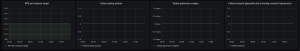
We therefore created this dashboard:

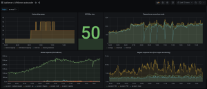
The dashboard reports everything we need to know about our PoP:

• Current autoscaling group state.
• RPS per instance.
• Global RPS and response time.

We also added some metrics related to the autoscaler itself, which are useful for detecting potential issues.

For example, how should the autoscaler behave if a server becomes overloaded during a bot attack and can’t give us its request volume? This could be a source of potential errors that we need to take into account in our calculation.

Our priority is always to protect as much traffic as we can, so in this case, we accept that our autoscaler may be over-provisioning instances for a short period of time. We have also invested a fair bit of time to make our components as resilient as possible to overloading … but that’s a story for another day. 🙂

Decision-Making Buffers

As you can see on the first screenshot above, our solution initially flickered a bit between two desired capacity values when we were close to the limit.

For example, if we were using 1200 requests per second per instance as our threshold, and we observed 1210 requests per second, we would add an instance. If the traffic volume went back down to 1180 requests per second, we would remove one.

Constantly adding and removing instances was a little messy, so we needed a way to mitigate. We also wanted to avoid downscaling too quickly, since heavy attacks often have short periods of reduced activity before the bots come back with full force again.

We are now using two types of buffers:

1. Volume Buffer: The autoscaler will only add machines if the volume is 50 requests per second higher than our threshold, and remove them if it’s 50 requests lower.
2. Time Buffer (for Downscaling): The autoscaler will only downscale if no other up- or downscaling action has been taken in the last 10 minutes.

Slashing Application Warm-Up Time

In addition to the limitations related to CloudWatch metrics, we identified a constraint within our own application: the application warm-up time.

To correctly detect and block malicious bots at the edge, our API servers are using model referentials. These referentials are changing all the time, as our machine learning models keep identifying new bot patterns and churning out algorithm updates.

Until recently, the referentials were presented to our API servers in a binary format, requiring dedicated computing on each consumer instance. Whenever a new API server booted, it had to compile its own referential, based on these descriptions of the latest models, before it could start to filter traffic. This process could take up to a couple of minutes, and on rare occasions even more.

To reduce this warm-up time, we introduced an intermediary element in our architecture which builds API server-ready referentials based on the raw descriptions. Now, when a new API server boots, it no longer needs to build its own referential, it can just fetch the already-compiled description of the most updated blocking models. It will then be updated via patches every millisecond (using Kafka topics), as our models are continuously learning from both ongoing and new bot attacks.

The results went beyond our wildest expectations: The architecture change slashed our application warm-up time by an entire minute!

Step 4: Optimize Costs

The previous optimizations all have a cost. We sometimes need hundreds of extra instances in the space of a few minutes, which has immediate repercussions on our AWS bills. The next step was therefore to look for ways to optimize these costs.

The Pros & Cons of Spot Instances

Spot instances are on-demand AWS machines that are much cheaper than standard instances—the price difference can be as much as 60-80%. There’s a good reason for this, though: spot instances can be interrupted and reattributed to someone else at any moment, if there is demand for them at a higher price. It’s kind of like an auction: if you’re not the highest bidder, tough luck.

We still want to use spot instances in production, since they are so much cheaper. But if we lose a spot instance, we won’t get it back; another instance will be created to replace it, and this takes a bit of time.

To minimize the impact of such switches, our application must be able to fail without breaking everything. This is where our stateless architecture really starts to pay off! Our dev team also did a great job minimizing the impact on our application in the case of a loss of a server: On every POP, our application is placed behind a load balancer, and health checks ensure that any failing instance will be removed from the backend list of the load balancer.

An Optimized Mix of Machines

Another condition for using spot instances was that if we lost multiple instances simultaneously, we had to be able to replace them very quickly.

This time, it was AWS who recommended the solution: using different types of machines. Our machines are all of the same size, but they are of different types.

If we’re using, say, 100 instances of the same type, we may lose them all at once if someone else suddenly needs 200 machines of that specific type. AWS will retrieve all our instances at that POP if the other user is ready to pay more. And if we lose 100 instances at the same time, we’re in trouble.

Whenever we need to quickly add a lot of new instances, we therefore now request three different types of spot instances. This significantly reduces the risk of losing many instances at once, since it’s extremely unlikely that someone else will request exactly the same mix of machine types as us, simultaneously.

We initially considered using even more different types, but there are constraints: our application must work on all the types of servers, and they must have sufficient computing capacity. In the end, we identified 3 types that work, and we have never had a loss of servers that had a negative impact on our application in production.

On our autoscaling groups, we applied this configuration:

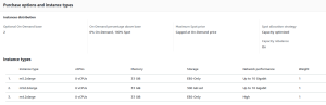
We have a base of two on-demand instances (the minimum for our autoscaling group), and the others are spot instances of three different types. Since m4.2xlarge is not available everywhere, some regions have only two instance types.

Step 5: Continuous Improvement

The homegrown autoscaler represented a breakthrough improvement in the performance of our infrastructure, but the job will never be completely done. We continue to measure, test and make incremental improvements to our infrastructure on a daily basis.

Minimizing Instance Boot Time

Instance boot time was one of the first areas we identified for potential further optimization.

When a scaling event is triggered (the autoscaler makes a request to AWS for a new instance), there is a small delay before the new instance becomes available to us, and there is also a small delay before our application starts on the new instance. During this time, the attack can change, and the instances we are already using may reach full capacity.

We can’t influence how quickly a new instance becomes available after the scaling event; this depends on AWS. So we decided to focus on minimizing the instance boot time, from the moment a scaling event is triggered and until our application is fully operational and can handle traffic on the new instance.

For this purpose, we tested and measured three different paths.

Operating System (AL2, Centos7, Centos8?)

One hypothesis was that our choice of operating system might influence the boot time. We were using Centos 7, so we tested Centos 8 and Amazon Linux 2 to see if either of them made any difference to the boot time.

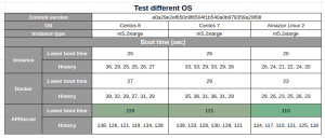
According to our tests, changing to Amazon Linux 2 would have enabled us to reduce the instance boot time by about 10 seconds. However, it would also have required a major development effort to introduce, and it wouldn’t be usable on our non-AWS POPs. Changing the distribution impacts core OS components, and can lead to huge differences in terms of behavior in production, making the debugging process more difficult.

We concluded that the 10-second improvement was not sufficient to justify the cost and inconvenience, and decided to keep Centos 7.

Instance Type

We also tested different instance types. When we request a new instance, we define how much storage, internal memory, and computing capacity we want. We were using m5.xlarge — would it help to use a smaller or larger type of server? For example, would the additional capacity of m5.2xlarge servers improve the instance boot time?

After testing all other m5 instances (and c5 as well), we found that the potential improvement was also just a few seconds, and the change was too costly. We decided to keep the m5.xlarge instance type.

Disk Size

Finally, we decided to experiment with the disk size of our EC2 instances. Historically, we have used 50GB EBS disks. But in fact, our application doesn’t store any files on the instance — so we don’t actually need this storage space.

After some tests on different instances, we discovered that indeed, the bigger the disk, the longer the boot time.

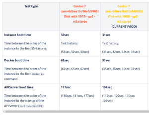
This was an extremely satisfying discovery: we were able to reduce the boot time by ~75 seconds just by using 8GB disks instead of 50GB! (We can’t go below 8GB, because if something goes wrong, the instance will start to write a bunch of files which we need a minimum of capacity to handle.)

Before this optimization, when we requested a new instance, it took approximately 2 – 2.5 minutes before our application was operational and could handle the incoming requests. Now, we have the right number of operational instances in 1.5 minutes. At any time, our infrastructure can handle the traffic we had 90 seconds ago — and it all happens automatically.

Customizing RAM

Our next objective is to increase the number of compatible instance types we can use. The purpose is to be able to spread our load over more additional types of servers, to reduce the risk of losing many spot instances at once (see the section “An optimized mix of machines” above).

The idea is to customize the RAM used by our Java application, based on the RAM which is available in a given instance. This should enable us to use bigger instances than we can today.

Our application currently works very well on 32GB RAM instances. We could make it work with 64GB instances, too, but this obviously has a cost.

Furthermore, when our application starts, it needs to understand the instance’s available RAM and attribute a suitable percentage of the RAM to itself. For example, the application must realize that there is 64GB RAM and use the entire capacity—it makes no sense for us to pay for a bigger machine if the application doesn’t use the full capacity. Conversely, if the instance has only 16GB RAM, the application must not start with the assumption that there is 32GB available.

At the time of writing, this optimization is not yet completed — stay tuned for the results!

Advanced Simulations

Finally, we’re exploring an avenue for improvement within the autoscaler itself: taking past metrics into account.

Today, the autoscaler reacts only to the latest metrics. For example, 120 > 100 = add 10 hosts, 150 > 120 = add 20 hosts, etc.

Instead of this linear feedback, we could use a polynomial interpolation or perform more complex simulations based on the last Y metrics. This would enable us to anticipate not only the current growth of traffic, but also the traffic growth to come.

Takeaways

DataDome’s bot detection solution frequently handles huge traffic spikes which we cannot anticipate, due to the nature of our customers’ traffic. To optimize the efficiency of our machine learning detection at the edge, even during major bot attacks, we must be able to scale our computing capacity as quickly as possible, at any time of the day or night.

Because of these real-time challenges, using CloudWatch metrics became a limiting factor. We decided to base our scaling decisions on a metric from our own application—requests per second (RPS)—instead of waiting for CloudWatch to analyze our ASC or NLB metrics and trigger the scaling operation.

To replace CloudWatch for scaling decisions, we developed an in-house application which now makes a decision every second. With further optimizations, we can now have all the instances we need available and fully operational within 90 seconds after the first sign of a traffic increase. Whether we need to multiply our capacity by 2 or by 200, it’s all fully automated.

• Challenge your existing stack, including low-level components.
• Don’t suppose; assess. Be data-driven and monitor your pains and your progress.
• Don’t over-engineer. Use simple tools first (here: CloudWatch), and assess their limits.
• Identify bottlenecks. Replace limited components. Develop them in-house if needed.
• Identify sources of costs, and monitor and optimize for the long term (FinOps).
• Plan for continuous improvements.